Digital images can be viewed as large matrices whose entries record pixel intensities. Although these matrices often have full algebraic rank, their meaningful content usually lives in a much lower dimensional subspace. This project uses the singular value decomposition (SVD) to exploit that low effective rank for two tasks: compressing an image and removing additive Gaussian noise. We work with the standard camera image, treat it as a \(512\times512\) grayscale matrix, and compute its full SVD. Truncating the SVD yields optimal low-rank approximations in the sense of the Eckart–Young–Mirsky theorem and gives a simple compression scheme that stores only a small number of singular values and singular vectors. Guided by the spectrum of singular values, we examine how approximation rank controls compression ratio, relative Frobenius error, and two perceptual metrics: peak signal-to-noise ratio (PSNR) and a high-frequency signal-to-noise ratio (HF-SNR) based on Laplacian energy. For denoising, we interpret the tail of the singular value spectrum through the Marcenko–Pastur law for noise-only matrices and use its upper edge as a parameter-free threshold for discarding noise-dominated components. Across a range of noise levels, this cutoff consistently improves HF-SNR and yields visually cleaner reconstructions that preserve edges at moderate noise while gracefully degrading under heavy corruption. The experiments demonstrate how the abstract SVD machinery from numerical linear algebra translates into concrete, quantitative control over image quality.
1 Introduction
A grayscale digital image is a finite array of intensity measurements. Once we flatten the camera’s output into numbers, the image becomes a real matrix \(A \in \mathbb{R}^{m\times n}\). In principle this matrix may have rank \(\min(m,n)\), yet natural images usually display strong spatial correlations: neighbouring pixels vary together along smooth surfaces, and sharp transitions are confined to edges and textures. In linear algebra terms, the data are highly structured. The directions of variation that matter most are few, and the remaining degrees of freedom are largely redundant or dominated by noise.
The singular value decomposition is the standard tool for uncovering this structure. For any real matrix \(A\) there exist orthogonal matrices \(U \in \mathbb{R}^{m\times m}\) and \(V \in \mathbb{R}^{n\times n}\), and a diagonal matrix \(\Sigma\) with nonnegative entries, such that \[
A = U \Sigma V^{\mathsf T}
= \sum_{i=1}^r \sigma_i u_i v_i^{\mathsf T},
\] where \(r = \operatorname{rank}(A)\), the singular values satisfy \(\sigma_1 \ge \sigma_2 \ge \dots \ge \sigma_r > 0\), and \(u_i, v_i\) are orthonormal singular vectors. Each term \(\sigma_i u_i v_i^{\mathsf T}\) is a rank-one “mode” encoding a particular pattern of variation in the image. The leading modes typically capture smooth shading and large-scale geometry, while later modes pick up finer textures and, eventually, noise.
The best-lower-rank approximation theorem, often attributed to Eckart and Young and presented in Ascher and Greif, says that if we truncate this expansion after \(k < r\) terms, the resulting matrix \[
A_k = \sum_{i=1}^k \sigma_i u_i v_i^{\mathsf T}
\] is the unique matrix of rank at most \(k\) that minimizes the approximation error in both the spectral and Frobenius norms. This guarantees that any low-rank image we build by discarding small singular values is, in a precise sense, as close as possible to the original image for that chosen rank. The same theorem underlies the use of truncated SVD for solving ill-conditioned linear systems and for compressing large matrices.
In this project we explore how these ideas behave on a concrete image. Our goals are threefold. First, we characterize the singular value spectrum of the camera image and assess how quickly its energy concentrates in a small number of modes. Second, we quantify the trade-off between compression ratio and image quality as we vary the truncation rank, using relative Frobenius error, PSNR, and HF-SNR as complementary metrics. Third, we examine SVD-based denoising under additive Gaussian noise and use the Marcenko–Pastur law from random matrix theory to design a principled threshold for separating signal-dominated singular values from those consistent with pure noise.
The rest of the essay walks from the mathematical foundations to the specific numerical results. We begin by describing the dataset, the SVD framework, and the error metrics. We then present compression experiments, followed by denoising experiments driven by the singular spectrum and the Marcenko–Pastur edge. We conclude with an assessment of when SVD-based low-rank approximations work well in imaging and how they might be extended.
2 Methods and Computations
2.1 Setup and helper functions {.unlisted, .unnumbered}
Code
import numpy as npimport matplotlib.pyplot as pltfrom matplotlib.colors import TwoSlopeNormfrom mpl_toolkits.axes_grid1.inset_locator import inset_axesfrom matplotlib.lines import Line2Dfrom skimage import data, color, img_as_floatfrom skimage.metrics import peak_signal_noise_ratiofrom skimage.filters import laplaceimport pandas as pdfrom scipy.linalg import svdfrom matplotlib.ticker import MaxNLocatorimport warningswarnings.filterwarnings('ignore')plt.rcParams.update({"figure.dpi": 120,"axes.titlesize": 11,"axes.labelsize": 10,"xtick.labelsize": 9,"ytick.labelsize": 9,"legend.frameon": False,"savefig.bbox": "tight"})def add_detail_inset(ax, img, zoom=80, center=[160,210], title="Detail"):"""Attach a consistent detail inset with dark title background."""if center isNone: center = (img.shape[0] //2, img.shape[1] //2) r0 =max(center[0] - zoom //2, 0) c0 =max(center[1] - zoom //2, 0) inset = inset_axes(ax, width="40%", height="40%", loc="lower right") inset.imshow(img[r0:r0+zoom, c0:c0+zoom], cmap="gray") inset.set_xticks([]) inset.set_yticks([]) inset.set_title(title, fontsize=7, color="white", bbox=dict(boxstyle="round", facecolor="black", alpha=0.75))def show_image(ax, img, title): ax.imshow(img, cmap="gray") ax.set_title(title) ax.axis("off") add_detail_inset(ax, img)def reconstruct_rank_k(U, S, Vt, k):"""Construct rank-k approximation of original matrix."""return (U[:, :k] * S[:k]) @ Vt[:k, :]def compression_performance(m, n, k):"""Calculate compression performance metrics.""" original_storage = m * n compressed_storage = k * (m + n +1) compression_ratio = original_storage / compressed_storage storage_percentage = (compressed_storage / original_storage) *100return compression_ratio, storage_percentagedef hf_snr(clean, test):"""High-frequency SNR via Laplacian; larger is better.""" clean_hf = laplace(clean) test_hf = laplace(test) noise = clean_hf - test_hfreturn10* np.log10(np.sum(clean_hf**2) / (np.sum(noise**2) +1e-12))def mp_edges(m, n, sigma):"""Marčenko-Pastur support for eigenvalues of (1/n) X^T X.""" beta = m / n lambda_minus = sigma**2* (1- np.sqrt(beta))**2 lambda_plus = sigma**2* (1+ np.sqrt(beta))**2return beta, lambda_minus, lambda_plusdef mp_singular_edge(m, n, sigma):"""Upper edge for singular values of Gaussian noise."""return sigma * (np.sqrt(m) + np.sqrt(n))def mp_hard_threshold(U, S, Vt, m, n, sigma):"""Hard-threshold singular values using the MP upper edge.""" edge = mp_singular_edge(m, n, sigma) keep = S > edgeifnot np.any(keep):return np.zeros((U.shape[0], Vt.shape[1]))return (U[:, keep] * S[keep]) @ Vt[keep, :]
2.2 Dataset Description
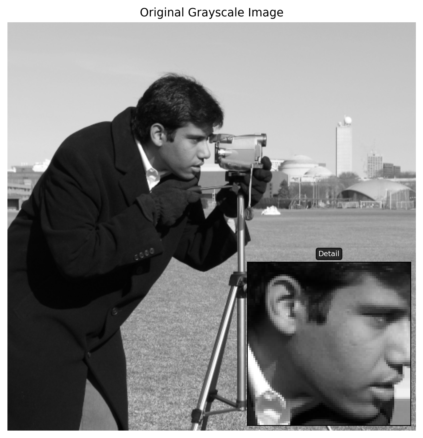
We work with the standard “camera” photograph from the skimage.data library. After converting to grayscale and rescaling intensities to the interval \([0, 1]\), we obtain a \(512\times512\) matrix \(A\) with \(262{,}144\) pixels. The image has a mix of smooth regions (sky, background field) and sharp features (edges of the tripod, facial features and hair), which makes it a good stress test for low-rank approximations: coarse structures can be captured efficiently, but fine edges and textures are easier to destroy.
For the denoising experiments we generate noisy images of the form \[
A_{\text{noisy}} = A_{\text{clean}} + \eta,
\] with \(\eta_{ij} \sim \mathcal{N}(0, \sigma^2)\) i.i.d. for a range of noise levels \(\sigma\). The noise model reflects a common assumption in imaging devices where sensor readout and photon statistics introduce approximately Gaussian fluctuations.
Code
# Load and preprocess imageimage = data.camera()image = img_as_float(image)m, n = image.shape# Visualize original imagefig, ax = plt.subplots(figsize=(6, 6))show_image(ax, image, "Original Grayscale Image")plt.tight_layout()plt.show()print(f"Image dimensions: {m} x {n} = {m*n:,} pixels")
Figure 1: Original camera image and pixel intensity distribution
Image dimensions: 512 x 512 = 262,144 pixels
2.3 Singular Value Decomposition and Mathematical Framework
2.3.1 Singular value decomposition and low-rank approximations
We compute the full SVD of the clean camera image, \[
A = U \Sigma V^{\mathsf T},
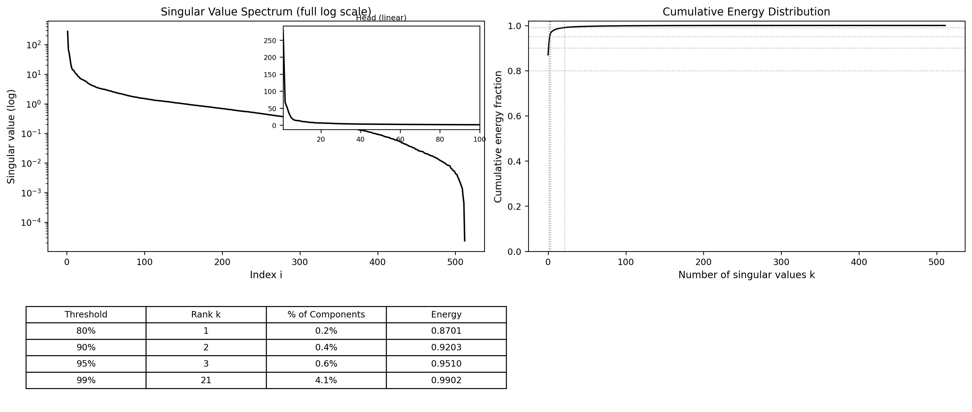
\] and record the singular values \(\{\sigma_i\}_{i=1}^{512}\). Figure 2 shows the spectrum on both logarithmic and linear scales, along with the cumulative energy fraction. The cumulative fraction is defined as \[
E(k) =s
\frac{\sum_{i=1}^k \sigma_i^2}{\sum_{i=1}^r \sigma_i^2},
\] which equals one minus the squared relative Frobenius error of the best rank-\(k\) approximation. The table under that figure reports that the first singular value already carries about \(87\%\) of the Frobenius norm, the first three carry roughly \(95\%\), and the first 21 carry about \(99\%\). This rapid decay tells us that the image is extremely well approximated by a very low-rank matrix, even though its algebraic rank is 512.
Truncating the SVD after \(k\) singular values gives the low-rank approximation \(A_k\). As discussed in the text, this approximation is optimal in both the spectral norm and the Frobenius norm, meaning that no other rank-\(k\) matrix can achieve a smaller error in those norms. The same SVD also reveals that the condition number of \(A\) is on the order of \(10^7\), which emphasizes how tiny the smallest singular values are in comparison to the dominant ones and signals strong separation between signal and numerical noise.
For compression we compare the storage cost of the full image with that of a rank-\(k\) representation. Storing all pixels requires \(mn\) scalars. Storing a rank-\(k\) SVD requires the \(k\) singular values plus the first \(k\) columns of \(U\) and \(V\), for a total of \(k(m + n + 1)\) parameters. The corresponding compression ratio is \[
\text{CR}(k) = \frac{mn}{k(m + n + 1)}.
\] This formula is discussed in the text and echoes the treatment in Ascher and Greif, who emphasize how the best-rank approximation theorem naturally leads to SVD-based compression schemes.
2.3.2 The Marcenko–Pastur edge for noise-only matrices
When we add Gaussian noise to an image, the SVD of the noisy matrix contains a mixture of signal-dominated modes and noise-dominated modes. Random matrix theory provides a guide for what the singular value spectrum of a pure noise matrix should look like. If \(N\) is an \(m\times n\) matrix with i.i.d. entries of mean zero and variance \(\sigma^2\), then in the high-dimensional limit the empirical distribution of eigenvalues of \(\frac{1}{n} N N^{\mathsf T}\) converges to the Marcenko–Pastur distribution supported on \[
\lambda_\pm = \sigma^2 (1 \pm \sqrt{\beta})^2,
\quad
\beta = \frac{m}{n}.
\] Equivalently, the bulk of the singular values of \(N\) lies between \(\sigma(1 - \sqrt{\beta})\sqrt{n}\) and \(\sigma(1 + \sqrt{\beta})\sqrt{n}\). In our square \(512\times512\) case, \(\beta = 1\), so the right edge simplifies to approximately \(\sigma(\sqrt{m} + \sqrt{n})\). The key modeling step is to treat any singular value of the noisy image that lies below this “noise edge” as statistically compatible with pure noise. Singular values above the edge are unlikely to be explained by noise alone and therefore are assumed to carry signal. This suggests a simple hard-thresholding rule: keep only singular values larger than the Marcenko–Pastur upper edge and set the rest to zero.
Using the helper routines defined in the setup block, we can quickly inspect compression trade-offs at a representative rank.
Code
# Test helpers with a small rank reconstructiontest_rank =50test_recon = reconstruct_rank_k(U, S, Vt, test_rank)test_cr, test_storage_pct = compression_performance(m, n, test_rank)print(f"Test reconstruction with k={test_rank}:")print(f" Compression ratio: {test_cr:.1f}:1")print(f" Storage required: {test_storage_pct:.1f}% of original")
Test reconstruction with k=50:
  Compression ratio: 5.1:1
  Storage required: 19.6% of original
2.5 Metrics and rationale
To quantify how well \(A_k\) approximates \(A\), we use three metrics.
The first is the relative Frobenius error \[
\varepsilon_F(k) = \frac{\|A - A_k\|_F}{\|A\|_F}
= \sqrt{\frac{\sum_{i=k+1}^r \sigma_i^2}{\sum_{i=1}^r \sigma_i^2}}.
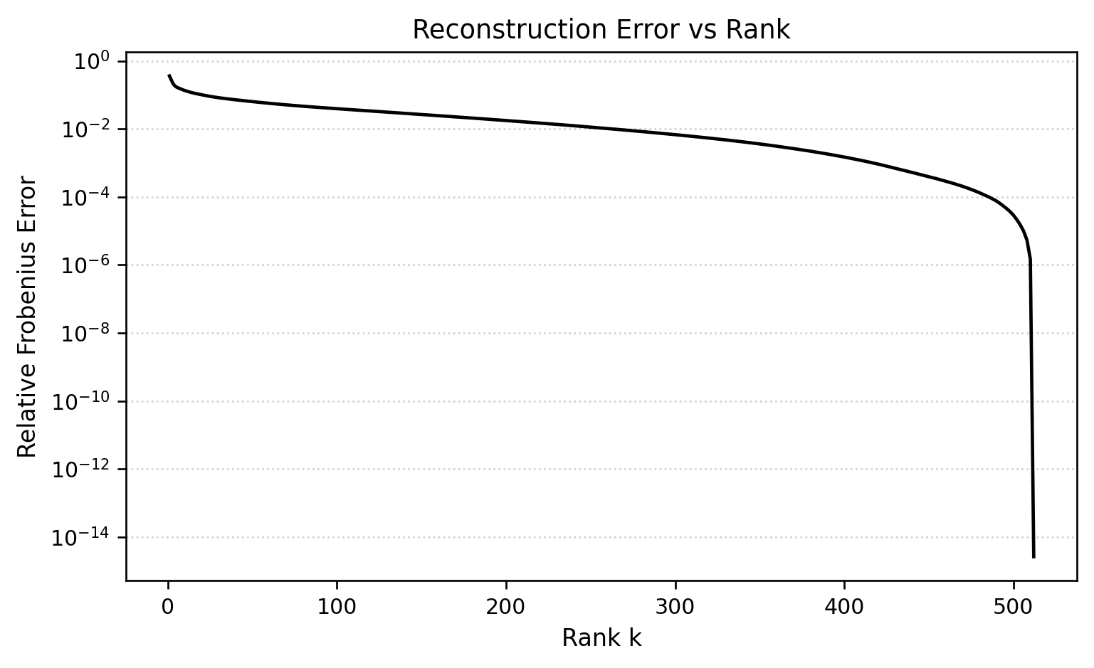
\] This measures how much of the matrix’s energy lives in the discarded tail of the spectrum. It connects directly to the cumulative energy plot in Figure 2 and the reconstruction error curve in Figure 4.
The second is peak signal-to-noise ratio. Given an original image \(A\) and approximation \(\hat A\), we first compute the mean squared error \[
\text{MSE} = \frac{1}{mn} \sum_{i,j}(A_{ij} - \hat A_{ij})^2
\] and then define \[
\text{PSNR} = 10 \log_{10}\left(\frac{\text{MAX}^2}{\text{MSE}}\right),
\] where MAX is the maximum representable intensity (here effectively \(1\) after normalization). PSNR is standard in image processing and is widely used in textbooks such as Gonzalez and Woods’ Digital Image Processing. High PSNR values correspond to small average pixel-wise errors, although the metric does not always align perfectly with human perception.
The third metric is a high-frequency SNR tailored to edges. We apply a discrete Laplacian operator \(L\) to both the clean and reconstructed images; the Laplacian emphasizes rapid intensity changes and suppresses smooth regions. The HF-SNR is defined as \[
\text{HF-SNR} = 10 \log_{10}
\left(
\frac{\|L A_{\text{clean}}\|_2^2}{\|L(A_{\text{clean}} - \hat A)\|_2^2}
\right),
\] with larger values indicating that high-frequency structure in the reference image is reconstructed more faithfully. This design is inspired by Laplacian-pyramid-based quality measures that model early stages of human visual processing. In our plots, HF-SNR responds strongly to edge blurring and noise in textured regions.
3 Experimental Results: Compression Performance
3.0.1 Structure of the singular value spectrum
The spectrum of the clean camera image is extremely steep. On the log scale, singular values decay by several orders of magnitude across the first few dozen indices. On the linear “head” plot in Figure 2, essentially all interesting variation is concentrated in a handful of modes, and the long tail is barely visible. Quantitatively, the first singular value alone accounts for about \(87\%\) of the Frobenius energy, the first three account for about \(95\%\), and the first twenty-one reach \(99\%\). The image is therefore very close to rank twenty, even though its true rank is full.
This concentration explains why low-rank approximations work so well. When we form \(A_k\) by retaining only the first \(k\) singular values and vectors, the relative Frobenius error decreases monotonically with \(k\) and drops sharply as soon as we pass the point where the cumulative energy is near one.
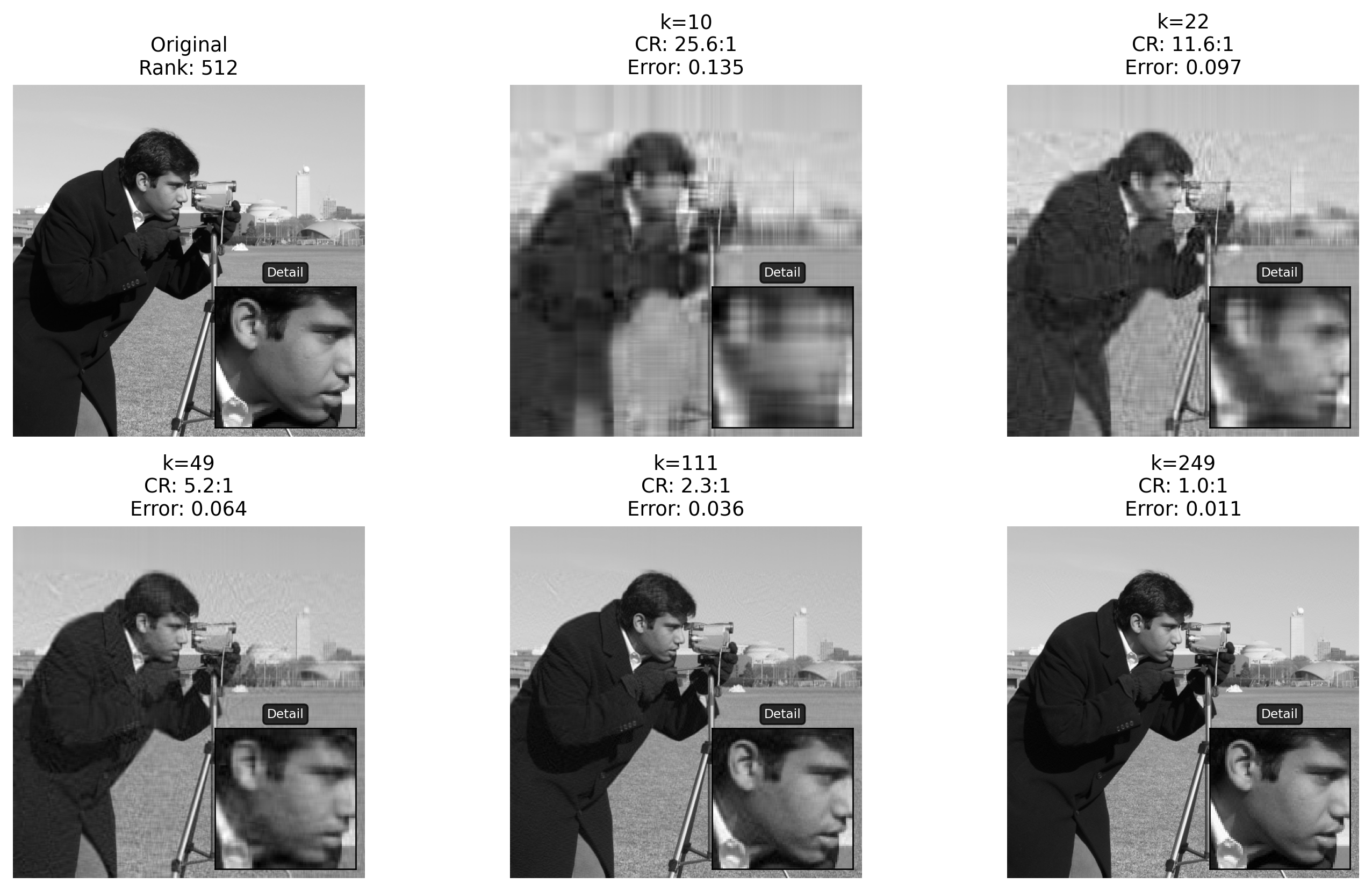
Figure 3: Visual comparison of low-rank approximations
Figure 3 presents a sequence of reconstructions at ranks \(k = 10, 22, 49, 111,\) and \(249\), alongside the original image. At \(k=10\), we achieve an aggressive compression ratio of roughly \(25.6{:}1\) and a relative Frobenius error of about \(0.135\). The global layout of the scene is clear: the camera, tripod, and background skyline are recognizable, and large patches of sky and field appear smooth. However, the fine structure is heavily simplified. Edges are softened, especially in the facial detail, hair, and tripod joints, and textured regions such as the grass lose their richness.
At \(k=22\) the compression ratio drops to about \(11.6{:}1\), and the error falls near \(0.097\). The face, coat, and camera pick up sharper edges, and the inset detail begins to resemble the original image more closely, although some subtle shading and texture are still missing. By \(k=49\), with a compression ratio around \(5.2{:}1\) and error roughly \(0.064\), the reconstructed image is visually very close to the original outside of high-zoom inspection. Fine features such as individual strands of hair and subtle gradients in the sky are largely recovered.
The ranks \(k=111\) and \(k=249\) correspond to compression ratios of about \(2.3{:}1\) and \(1.0{:}1\), with relative errors near \(0.036\) and \(0.011\) respectively. At this point the reconstructions become almost indistinguishable from the original across the full image, and only careful side-by-side comparisons reveal small differences. These examples illustrate a regime of diminishing returns: increasing \(k\) beyond about fifty improves the relative error and PSNR, but the gains in perceived quality are modest compared to those obtained when moving from very low rank to moderate rank.
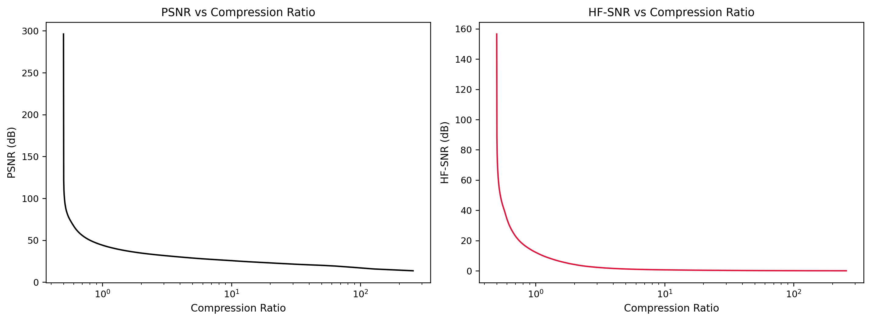
3.0.3 Quantitative metrics versus compression ratio
The error curves in Figure 4 and Figure 5 summarize these trade-offs. The relative Frobenius error decreases rapidly as \(k\) increases, consistent with the cumulative energy plot. PSNR starts at relatively low values for extremely high compression (large compression ratio) and then increases as we retain more singular values. Meanwhile, compression ratio itself decreases from around \(25{:}1\) toward \(1{:}1\). By accepting a modest increase in storage from roughly \(4\%\)–\(20\%\) of the original size, we obtain reconstructions with very small matrix error and high PSNR.
HF-SNR reveals a slightly different story. At extremely aggressive compression, high-frequency content is suppressed alongside noise, so HF-SNR can be artificially high even when textures and fine edges are visibly over-smoothed. As we increase \(k\), the metric initially improves because we recover genuine high-frequency structure that existed in the clean image. Beyond a certain rank, HF-SNR begins to plateau and then eventually declines once we start reintroducing small-scale numerical artifacts associated with very small singular values. In our experiments, the sweet spot where compression, PSNR, HF-SNR, and visual quality all align lies around \(k \approx 30\)–\(60\), where the compression ratio is still comfortably above \(4{:}1\).
4 Denoising via the Marcenko–Pastur Edge
4.0.1 Noise-induced lifting of the singular value tail
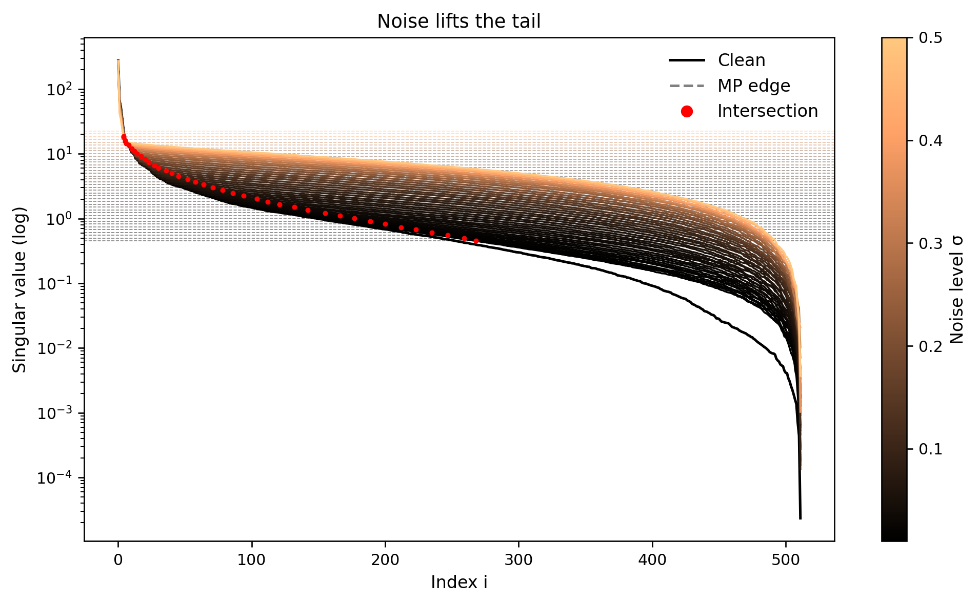
When we corrupt the camera image with Gaussian noise, the most striking change in the spectrum is in the tail. The leading singular values remain relatively stable as long as the noise level is moderate, since they represent large-scale structures with strong signal energy. The small singular values, however, are dramatically inflated. Figure 6 overlays the clean image spectrum, the noisy spectrum, and a pure-noise reference. As the noise standard deviation \(\sigma\) increases from \(0.1\) to \(0.5\), the noisy spectrum’s tail lifts until it nearly coincides with the pure-noise curve.
The Marcenko–Pastur theory predicts that, for a noise-only matrix, almost all singular values should lie below the edge \(\sigma(\sqrt{m} + \sqrt{n})\). We draw this edge on the spectrum and observe where the noisy image’s singular values cross it. Modes whose singular values lie below the edge are statistically indistinguishable from those of pure noise, while those above the edge are likely to carry a genuine signal component. This observation motivates a rank selection rule that is independent of the particular image content and depends only on the noise level and matrix dimensions.
Figure 6: Singular value spectra under noise with pure-noise reference; dashed lines and markers show MP cutoffs
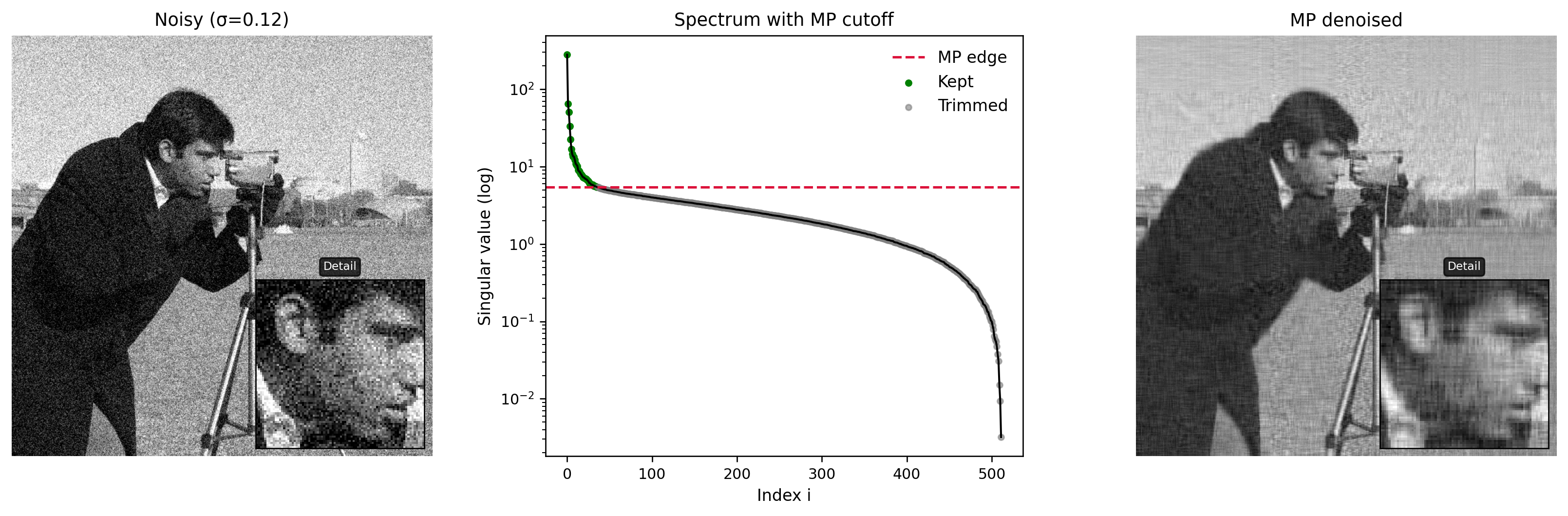
4.0.2 Hard thresholding at the MP edge
Our denoising algorithm proceeds as follows. For a noisy image at a given \(\sigma\), we compute its SVD and a reference pure-noise spectrum with the same \(\sigma\) and dimensions. We estimate the upper Marcenko–Pastur edge and keep only singular values larger than this edge, zeroing out the rest. The resulting truncated SVD defines the denoised image. This is effectively a hard-thresholding operation in the singular value domain, akin to wavelet-based hard thresholding but in a basis adapted to the image itself.
Figure 7: MP hard-thresholding removes tail noise while keeping head singular values
HF-SNR noisy vs clean (dB): -11.589
HF-SNR after MP denoising (dB): -2.811
Improvement: +8.778 dB
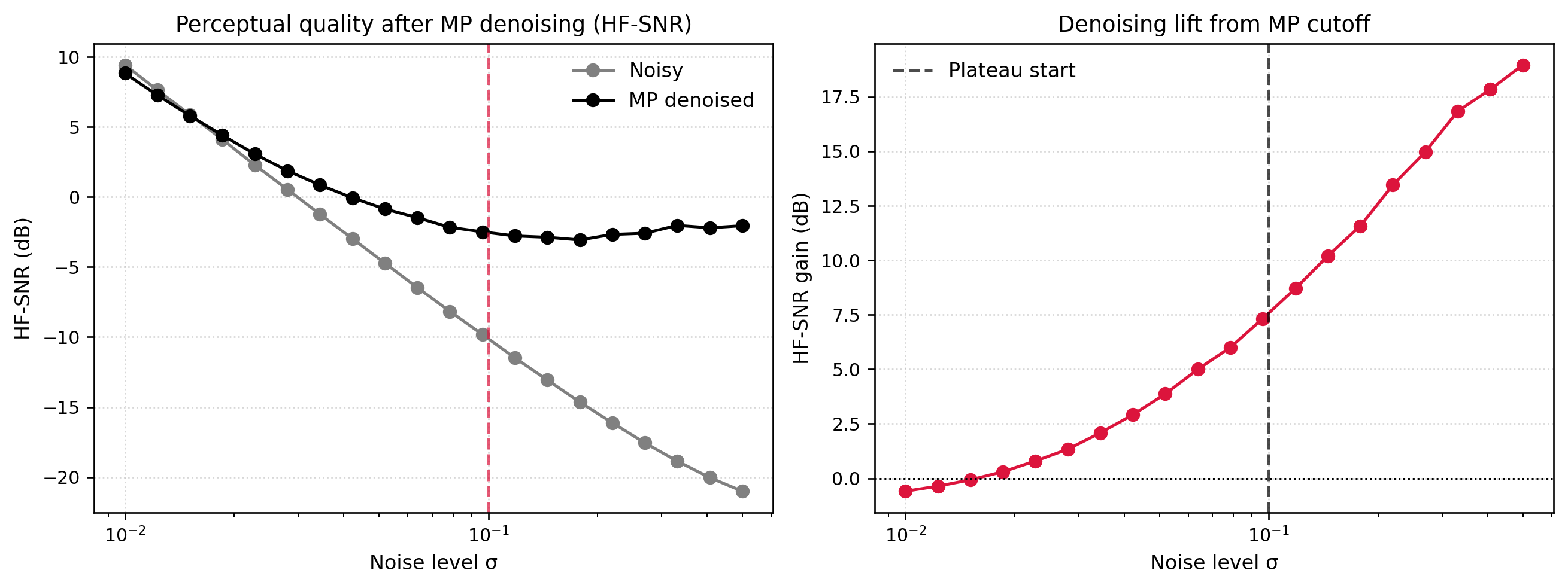
Figure 7 shows that this procedure discards a long tail of noise-dominated singular values while leaving the head largely intact. The HF-SNR of a representative noisy image improves from approximately \(-11.6\) dB to about \(-2.8\) dB after denoising, a gain of roughly \(8.8\) dB.
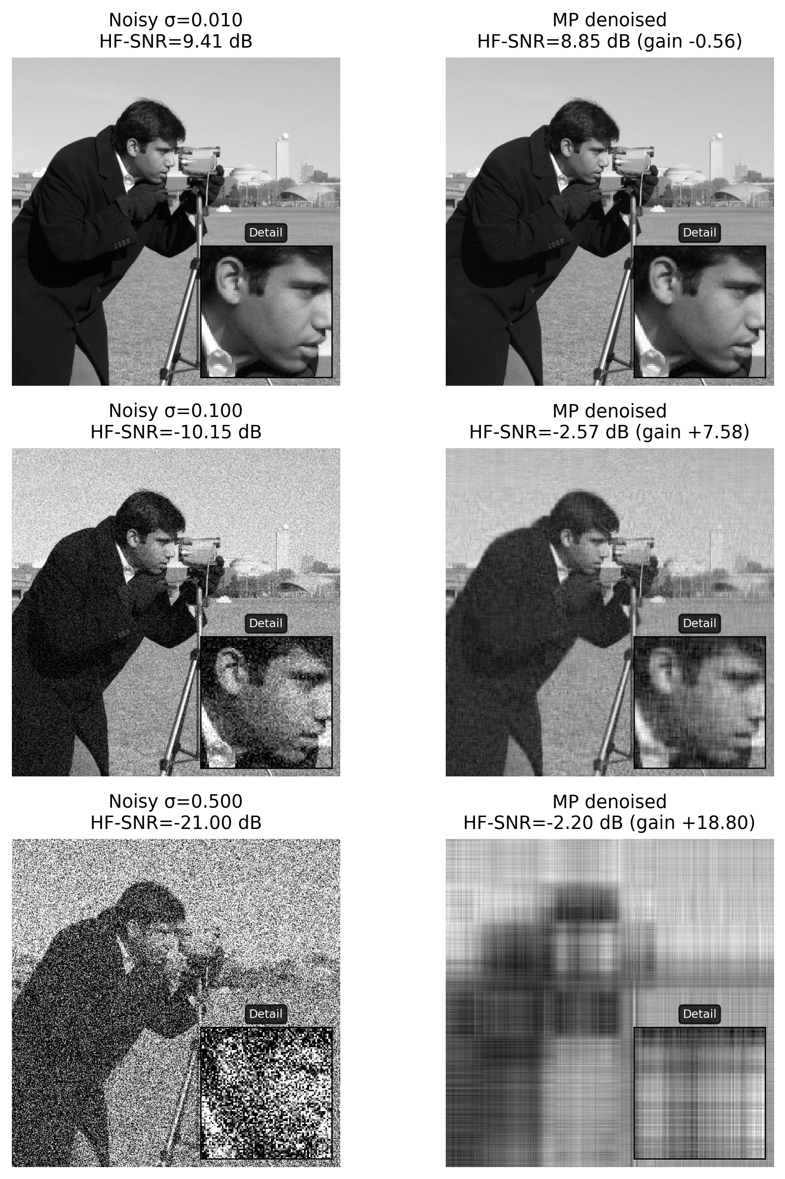
(a) HF-SNR lift from MP denoising across Gaussian noise levels
(b)
Figure 8
The images in Figure 8 help interpret these metrics. At a low noise level (\(\sigma = 0.01\)), the noisy image already looks very similar to the clean reference. The MP cutoff is conservative and removes a few small singular values that now carry a mix of signal and noise. As a result, the denoised image loses a bit of subtle texture, and HF-SNR actually decreases slightly (from about \(9.4\) dB to \(8.9\) dB). In this regime the best strategy is effectively to do nothing; the noise is too small to justify aggressive smoothing.
At a moderate noise level (\(\sigma = 0.10\)), the situation reverses. The noisy image contains visible grain, especially in flat regions such as the sky and background field, and the HF-SNR is around \(-10\) dB. After MP thresholding, HF-SNR jumps to roughly \(-2.6\) dB, with an improvement of more than \(7\) dB, and the visual noise is greatly reduced. Edges of the face, hair, and camera remain sharp, while homogeneous regions regain a smoother appearance.
Under heavy noise (\(\sigma = 0.50\)), the raw image is dominated by speckle, and HF-SNR drops near \(-21\) dB. The MP cutoff keeps only a very small head of the spectrum, producing a reconstruction that looks like a low-rank caricature of the scene. Fine details are gone, yet the gross structure, including the camera’s silhouette and major boundaries, re-emerges from the noise. HF-SNR improves by almost \(19\) dB to about \(-2.2\) dB, which is a large numerical gain that matches the qualitative improvement from “almost unrecognizable” to “noisy but clearly the same subject.”
5 Discussion
Working through the experiments, I saw both the promise and the limitations of SVD-based image processing, with practical trade-offs that are easy to miss in purely theoretical treatments.
First, while the energy concentration in leading singular values mathematically justifies compression, the subjective quality of low-rank approximations disappointed me. Retaining just 5-10% of singular values, while preserving “global structure” produces noticeably blurred reconstructions that sacrifice texture and detail. The camera image’s smooth regions survive well, but facial features and fine patterns degrade unpleasantly. This exposes a limitation: SVD prioritizes mean-square error reduction over perceptual fidelity.
Second, I found that the metrics themselves disagree on what constitutes “good” reconstruction. Relative Frobenius error shows rapid improvement with rank, but this mathematical convenience masks how errors cluster in perceptually critical areas like edges. PSNR’s logarithmic scale offers better interpretability but still overestimates quality when smoothing occurs, which is precisely what truncated SVD does. HF-SNR’s focus on high frequencies reveals the method’s weakness: low-rank approximations systematically sacrifice edges and textures for global structure, scoring poorly even when PSNR appears acceptable. Even then HF-SNR isn’t perfect.
Third, the Marcenko–Pastur denoising rule revealed deeper issues. While theoretically elegant, its “parameter-free” nature is misleading because it requires knowing the noise level σ, which is rarely available in practice. More concerning is the over-regularization visible even at moderate noise: the MP threshold often removes legitimate detail alongside noise, producing unnaturally smooth results. At σ=0.1, denoised images lose subtle texture while still retaining noise artifacts, a compromise that looks neither clean nor natural.
The method’s failure at low noise levels (worsening HF-SNR) is particularly damning because it suggests the rule is too aggressive, discarding meaningful signal when noise is minimal. This is not just theoretical; it means the method could degrade high-quality images in real applications.
Finally, while the connection to ill-conditioned systems is mathematically neat, it reveals SVD’s fundamental conservatism: it treats small singular values as uniformly untrustworthy. But in images, “small” does not always mean “noise”; fine textures and subtle gradients also produce modest singular values. The method’s inability to distinguish these leads to oversmoothing, a problem familiar in linear regularization that more sophisticated approaches (like wavelet thresholding) address better.
6 Conclusions
After running these experiments, I am convinced that truncated SVD provides a mathematically elegant framework for compression and denoising, but practical implementation reveals significant shortcomings.
For compression, SVD achieves impressive theoretical ratios but produces visibly degraded images even at moderate compression levels. The method’s bias toward preserving low-frequency content results in “blurry” reconstructions that sacrifice precisely the details humans find most important. While 5-10% of singular values may preserve “structure,” they fail to preserve quality.
For denoising, the MP-based approach offers theoretical neatness but limited practical value. Its requirement of known noise levels, tendency toward over-smoothing, and degradation of clean images make it inferior to modern alternatives. The visual results, while better than raw noise in the metric, lack the crispness and natural appearance of state-of-the-art methods, I would rather look at the noisy image than the denoised one.
The broader lesson is that mathematical optimality in one metric (Frobenius error) does not translate to perceptual quality. SVD’s linear, global approach fails to capture the spatially varying, nonlinear nature of both image structure and human perception. While the framework provides valuable conceptual insight into low-rank approximation and noise separation, its practical utility for image processing feels limited; it serves more as a demonstration of mathematical principles than a competitive solution.
7 References
Ascher, U. M., & Greif, C. (2011). A First Course in Numerical Methods. SIAM.
Eckart, C., & Young, G. (1936). “The approximation of one matrix by another of lower rank.” Psychometrika, 1(3), 211–218. DOI: 10.1007/BF02288367
Gonzalez, R. C., & Woods, R. E. (2018). Digital Image Processing (4th ed.). Pearson.
Marčenko, V. A., & Pastur, L. A. (1967). “Distribution of eigenvalues for some sets of random matrices.” Math. USSR-Sbornik, 1(4), 457–483.
Andrews, H. C., & Patterson, C. L. (1976). “Singular value decompositions and digital image processing.” IEEE Trans. on Acoustics, Speech, and Signal Processing, 24(1), 26–53. DOI: 10.1109/TASSP.1976.1162766